Last week I studied and practiced Python programming from Codeacademy's online Python Course. This is a really nice, easy to follow and interactive course. Estimated course time is 13 hours but it took me nearly 26 hours to finish. After finishing the course, I decided to analyze data using Python to familiarize myself with Python's Data Analysis Library: Pandas, Scientific Computing Libraries : NumPy, SciPy, Plotting Library: matplotlib (IMO: ggplot2 package in R plots much better looking plots compared to matplotlib plots), and scikit-learn for Machine Learning in Python.
For analyzing data I am using Titanic: Machine Learning from Disaster data from Kaggle's knowledge based competition, a major reason to use this data is that there are a lot of online Python tutorials and blogs that use this data and this makes learning/understanding easier.
Note: This is not a tutorial. The data analysis done here is based on various online Titanic Data related Python tutorials/blogs.
#############################################################
### Kaggle Competition: Titanic Machine Learning from Disaster
# Import important libraries and modules
import matplotlib.pyplot as plt
import numpy as np
import pandas as pd
import pylab as p
import sklearn as sol
# Reading Titanic (training) data
train = pd.read_csv("/Users/Ankoor/Desktop/Python/Kaggle/Titanic/train.csv")
# View dataframe
train
# View first 'n' rows (R*)
train.head(5)
Out:
train.tail(3)
# Get column names (features / attributes) in data frame [Similar to R's names()]
list(train)
Out:

# What kind of data array is 'train'?
type(train)
Out: pandas.core.frame.DataFrame
train.dtypes
PassengerId int64
Survived int64
Pclass int64
Name object
Sex object
Age float64
SibSp int64
Parch int64
Ticket object
Fare float64
Cabin object
Embarked object
dtype: object
train.info()
Out:

There are 891 observations. Features 'Age' (714 observations remaining), 'Cabin' (204 observations remaining) and 'Embarked' (889 observations remaining) have missing data.
# Checking missing values in the data: Age and Cabin
sum(train['Age'].isnull())
Out: 177
177 'Age' observations missing
sum(train['Cabin'].isnull())
Out: 687
687 'Cabin' observations missing
Note: .isnull() does not work for 'str'
# Describe data: Count, Mean, STD, Min, Max [Similar to R's summary()]
train.describe()
Out:

train['Age'][0:10]
Out:

train.Age[0:10]
# Type of referenced data?
type(train['Age'])
type(train.Age) # another command to get type of referenced data
# Mean Age (Ignoring missing values)
train.Age.mean()
train['Age'].mean()
Out: 29.69911764705882
# Median Fare (Ignoring missing values)
train.Fare.median()
train['Fare'].median()
Out: 14.4542
# Unique values
train.Sex.unique()
Out: array(['male', 'female'], dtype=object)
train['Embarked'].unique()
Out: array(['S', 'C', 'Q', nan], dtype=object)
train['Pclass'].unique()
Out: array([3, 1, 2])
3 Passenger classes
train[['Sex', 'Pclass', 'Age']]

train[train['Age'] > 60]
Out:

train[train['Age'] > 60][['Sex', 'Pclass', 'Age', 'Survived']]
Out:

# Filtering and sub-setting data with missing values
train[train['Age'].isnull()][['Sex', 'Pclass', 'Age', 'Survived']]
# Counting # of males in each passenger class
for i in range(1, 4):
print i, len(train[(train['Sex'] == 'male') & (train['Pclass'] == i)])
Out:
1 122
2 108
3 347
# Counting # of females in each passenger class
for i in range(1, 4):
print i, len(train[(train['Sex'] == 'female') & (train['Pclass'] == i)])
Out:
1 94
2 76
3 144
# Simple Histogram of Age
train['Age'].hist()
p.show()
Out:

# Histogram of Age (after dropping missing values), alpha controls 'transparency'?
train['Age'].dropna().hist(bins = 16, range = (0, 80), alpha = 0.5)
Out:


## Cleaning data: Transforming 'String values'
# 1. Adding a new column and filling it with a number
train['Gender'] = 4
# 2. Populating the new column 'Gender' with M or F
train['Gender'] = train['Sex'].map(lambda x: x[0].upper())
# 3. Populating the new column witn binary integers
train['Gender'] = train['Sex'].map({'female': 0, 'male': 1}).astype(int)
## Feature Engineering: Name attribute has honorific titles like Mr., Mrs., etc
# Extracting salutation from Name (Format: Last Name, Title, First Name)
# Name example: Dahlberg, Miss. Gerda Ulrika
def title(name):
temp_1 = name.split(',') # Split by (,)
temp_2 = temp_1[1].split('.')[0] # Split by (.)
temp_3 = temp_2.strip() # Remove white space
return temp_3
train['Title'] = train['Name'].apply(title) # Apply function 'title' to 'Name'
train[['PassengerId', 'Survived', 'Sex', 'Pclass', 'Age', 'Gender', 'Title']]
Out:


## How to count passenger by Title
# Grouping by Title
temp_4 = train.groupby('Title')
# Counting passengers by Title
temp_5 = temp_4.PassengerId.count()
print temp_5
Out:


# Barplot: Passenger count by title
temp_5.plot(kind = 'bar')
Out:

Majority of passengers had 4 honorific titles: Mr, Mrs, Miss, and Master. I will rename (1) honorific titles like Capt, Don, Dr, Jonkheer, Major, Rev and Sir to Mr; (2) honorific titles like Lady, Mme, Ms, and the Countess to Mrs; (3) honorific titles like Mlle to Miss
# How many males and females are Doctors?
train[train['Title'] == 'Dr']
Out:
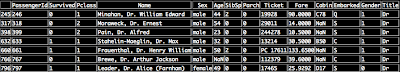

6 male doctors and 1 female doctor (Dr. Alice (Farnham) Leader)
## Create a 'Temp' column in train and fill it with concatenated 'Sex' and 'Title' string values
train ['Temp'] = train['Sex'] + train['Title']
## Replace concatenated value 'femaleDr' value with 'Mrs'
train.loc[train['Temp'] == 'femaleDr', 'Title'] = 'Mrs'
# Drop 'Temp' column
train = train.drop(['Temp'], axis = 1)
## There are 4 main titles: Mr, Mrs, Master and Miss, and some other titles
# Taking care of other titles
def new_title(title):
if title == 'Mr' or title == 'Capt' or title == 'Don' or title == 'Dr' or title == 'Jonkheer' or title == 'Major' or title == 'Rev' or title == 'Sir' or title == 'Col':
return 'Mr'
elif title == 'Mrs' or title == 'Lady' or title == 'Mme' or title == 'Ms' or title == 'the Countess':
return 'Mrs'
elif title == 'Miss' or title == 'Mlle':
return 'Miss'
else:
return 'Master'
train['NewTitle'] = train['Title'].apply(new_title)
# Drop 'Title' attribute
train = train.drop(['Title'], axis = 1)
# Grouping by Title
temp_6 = train.groupby('NewTitle')
# Counting passengers by Title
temp_7 = temp_6.PassengerId.count()
print temp_7
temp_7.plot(kind = 'bar')
temp_7.plot(kind = 'bar')
Out:


Out:


Now all the passenger honorific titles have been updated.
## Now descriptive statistics plots to understand data and survival chance
train.boxplot(column = 'Age', by = 'NewTitle')

Outliers: Miss with Age around 60? I used train[(train['Age'] > 30) & (train['NewTitle'] == 'Master')] and found that some females with age > 30 years have 'Miss in their title (May be they were unmarried or some other reason)
train.boxplot(column = 'Fare', by = 'Pclass')
Out:

Outliers: Some passengers in First Class have paid more than $200 for tickets, may be they have paid for their whole family.
# Passenger distribution by Passenger Class and Survival Chance
group_1 = train.groupby('Pclass').PassengerId.count()
group_1.plot(kind = 'bar')
Out:

Out:

Almost half of the passengers were 3rd class passengers
group_2 = train.groupby('Pclass').Survived.sum()
Pclass_Survival_Prob = group_2/group_1
Pclass_Survival_Prob.plot(kind = 'bar', color = 'pink', alpha = 0.65)
Out:
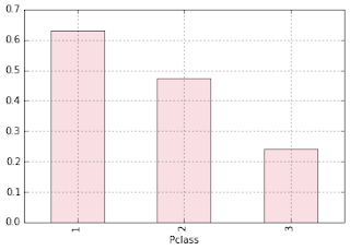
Out:

However, more First Class and Second Class passengers survived compared to passengers in Third Class (May be better access to Lifeboats/Life Jackets, or easy access to upper decks?)
# Passenger distribution by Passenger Class, Gender and Survival Chance
# Barplot using Cross-tabulation
group_3 = pd.crosstab([train.Pclass, train.Sex], train.Survived)
group_3.plot(kind = 'bar', stacked = True, color = ['black', 'yellow'])
Out:


group_5 = pd.crosstab([train.Pclass, train.NewTitle], train.Survived)
group_5.plot(kind = 'bar', stacked = True, color = ['black', 'yellow'])
Out:

group_6 = pd.crosstab([train.Embarked, train.NewTitle], train.Survived)
group_6.plot(kind = 'bar', stacked = True, color = ['black', 'yellow'])
Out:

Out:

Compared to males more females survived the disaster.
# Some other related plots
group_4 = pd.crosstab([train.Pclass, train.Sex, train.Embarked], train.Survived)
group_4.plot(kind = 'bar', stacked = True, color = ['black', 'yellow'], alpha = 0.5)
group_4.plot(kind = 'bar', stacked = True, color = ['black', 'yellow'], alpha = 0.5)
Out:

group_5.plot(kind = 'bar', stacked = True, color = ['black', 'yellow'])
Out:

group_6.plot(kind = 'bar', stacked = True, color = ['black', 'yellow'])
Out:

# Feature Engineering: Family size
train['Family'] = train['SibSp'] + train['Parch']
group_7 = pd.crosstab([train.Pclass, train.Family], train.Survived)
group_7.plot(kind = 'bar', stacked = True, color = ['black', 'yellow'], alpha = 0.25)
train['Family'] = train['SibSp'] + train['Parch']
group_7 = pd.crosstab([train.Pclass, train.Family], train.Survived)
group_7.plot(kind = 'bar', stacked = True, color = ['black', 'yellow'], alpha = 0.25)
## Imputing missing values in attribute 'Age'. I found the code used below at this blog.
# View dataframe: 'Age' = NaN
train[train['Age'].isnull()].head()
table = train.pivot_table(values = 'Age', index = ['NewTitle'], columns = ['Pclass', 'Sex'], aggfunc = np.mean)
def ageFunc(x):
return table[x['Pclass']][x['Sex']][x['NewTitle']]
train['Age'].fillna(train[train['Age'].isnull()].apply(ageFunc, axis = 1), inplace = True)
train['Age'] = train['Age'].astype(int)
#Some more plots
#Specifying Plot Parameters
# figsize = (x inches, y inches), dpi = n dots per inches
fig = plt.figure(figsize = (11, 8), dpi = 1600)
# Plot: 1
ax1 = fig.add_subplot(221) # .add_subplot(rcp): r = row, c = col, p = position
female_hiclass = train['Survived'][train['Sex'] == 'female'][train['Pclass'] != 3].value_counts()
female_hiclass.plot(kind = 'bar', label = 'Female High Class', color = 'deeppink', alpha = 0.25)
ax1.set_xticklabels(['Survived', 'Dead'], rotation = 0)
ax1.set_xlim(-1, len(female_hiclass))
ax1.set_ylim(0, 400)
plt.legend(loc = 'best')
# Plot: 2
ax2 = fig.add_subplot(222) # .add_subplot(rcp): r = row, c = col, p = position
female_loclass = train['Survived'][train['Sex'] == 'female'][train['Pclass'] == 3].value_counts()
female_loclass.plot(kind = 'bar', label = 'Female Low Class', color = 'pink', alpha = 0.25)
ax2.set_xticklabels(['Survived', 'Dead'], rotation = 0)
ax2.set_xlim([-1, len(female_loclass)])
ax2.set_ylim(0, 400)
plt.legend(loc = 'best')
# Plot: 3
ax3 = fig.add_subplot(223) # .add_subplot(rcp): r = row, c = col, p = position
male_hiclass = train['Survived'][train['Sex'] == 'male'][train['Pclass'] != 3].value_counts()
male_hiclass.plot(kind = 'bar', label = 'Male High Class', color = 'teal', alpha = 0.25)
ax3.set_xticklabels(['Dead', 'Survided'], rotation = 0)
ax3.set_xlim(-1, len(male_hiclass))
ax3.set_ylim(0, 400)
plt.legend(loc = 'best')
# Plot: 4
ax4 = fig.add_subplot(224) # .add_subplot(rcp): r = row, c = col, p = position
male_loclass = train['Survived'][train['Sex'] == 'male'][train['Pclass'] == 3].value_counts()
male_loclass.plot(kind = 'bar', label = 'Male Low Class', color = 'green', alpha = 0.25)
ax4.set_xticklabels(['Dead', 'Survived'], rotation = 0)
ax4.set_xlim(-1, len(male_loclass))
ax4.set_ylim(0, 400)
plt.legend(loc = 'best')
Out:

Females in the high class had better survival chance compared to females in low class. Irrespective of the class more male passengers perished compared to females.